Multibody Dynamics B
|
|
|
|
Delft University of Technology |
Description: After the first courses in dynamics a
student can often deal well with the dynamics of one rigid body.
In this course we will cover a systematic approach to the
generation and solution of equations of motion for mechanical
systems consisting of multiple interconnected rigid bodies, the
so-called multibody systems. This course differs from ``advanced
dynamics'', which mostly covers theoretical results about classes
of idealized systems (e.g. Hamiltonian systems), in that the goal
here is to find the motions of relatively realistic models of systems
(including, for example, motors, dissipation and contact
constraints).
The main approach is the reduction of the constraint Newton-Euler equations using the principle of virtual work and the principle of D'Alembert. However the relation of this approach to Lagrange's equations, Kane's equations, and to the differential algebraic equations approach will also be covered. The course will start with 2D examples and then move on to 3D systems. Rotations will be represented with matrices, various Euler angles, and Euler parameters. Various computer solution techniques for the ODEs or DAEs will also be covered.
Goal: By the end of the course students will be competent at finding the motions of linked rigid body systems in two and three dimensions including systems with various kinematic constraints (sliding, hinges and rolling, closed kinematic chains). Collisional interactions will be considered in a unified manner for all the different ways of formulating the equations of motion.
Homework: There will be weekly homework assignments and a final project. The homework is due a week after hand out and will be graded. Hand in your homework at the start of class at the front. The homework is strictly individual but in doing the homework I encourage you to work together within the rules and regulations.
Rule and Regulations:
To get credit, on every homework assignment
please do the following things:
-
On the top right corner neatly print the following, making appropriate substitutions as appropriate:
Sally Rogers, # 9123456
wb1443, HW#1
Due Thu Feb 15, 2007. -
At the top clearly acknowledge all help you got from Faculty, students, or ANY other source (but for lecture and text). Examples could be "Mary Jones pointed out to me that I needed to draw the second FBD in problem 2." or "Nadia Chow showed me how to do problem 3 from start to finish." or "I basically copied this solution from the posted solutions." etc. If I think you are taking too much from other sources I will tell you. In the mean time don't violate academic integrity rules: be clear about which parts of your presentation you did not do on your own. More on academic integrity see: http://www.cuinfo.cornell.edu/Academic/AIC.html..
-
All computer output should have your name clearly visible, as printed by the computer (e.g., title plots with your name, put your name in a comment in the first line of any .m files, etc.)
-
Your work should be laid out neatly enough to read by someone who does not know how to do the problem. Part of your job as an engineer is not just to get the right answer, but convincingly so. That is your job on the homework as well.
-
Be concise, don't burden the TA's with page after page of computer output (wallpaper) or lengthy derivations. Blaise Pascal (1623--1662) once wrote to a friend: "This letter is rather long, because I didn't have the time to make it shorter."
The graded work can be picked up at the end of class or at TA's office.
Grading: Total course grading is 70 % homework and 30 % final project. Homework is the average of the weekly homework assignments. Final project is the grading of the written report on the final project (strictly individual!).
News
-
Sep 10, 2013:
The Final Grades are now available, see:
wb1413-2013-FinalGrades.pdf
Please check your grades and report any problems to
me.
-28 March:
in-class quizzes with the TurningPoint software and voting via
Responseware, see below.
Hand-Outs
- The course
contents.
- Preliminary course notes, first few chapters
MultibodyDynamicsB.pdf.
- My lecture notes on numerical integration
NumericalIntegrationCh7.pdf
- My lecture notes on the coordinate projection method:wb1413_diktaatCh8.pdf
- My lecture notes: NotesFrom2DTo3D.pdf
- My lecture notes on 3D rotation:
wb1413_diktaatCh9.pdf
- One of my favourite papers on 3D rotation,
"How to...": DETC2006Paper99307.pdf
- Reprint from
Lanczos1949.
Homework
Assignment 1,
due
Thu 21 Feb 15:45 h.
Assignment
2,
due
Thu 07 Mar 15:45 h.
Assignment
3,
due
Thu 14 Mar 15:45 h.
Assignment
4,
due
Thu 28 Mar 15:45 h.
Assignment
5,
due
Mon 08 Apr 15:45 h.
Assignment
6,
due
Thu 02 May 15:45 h.
Assignment
7,
due
Mon 13 May 17:00 h.
Assignment
8, due Thu 23 May 15:45 h.
Assignment
9, due Thu 30 May 15:45 h.
Assignment
10, due Thu 6 June 15:45 h.
Final Project
Pick one of the final projects and hand-in your report on paper
Monday 1 July 2013 17:00 h the latest to me, Arend Schwab, in my paper mailbox.
- Final Project 1, Dynamic
analysis of an
Ejection Seat Reverse Bungee (average difficulty level).
- Final Project 2, Dynamic
analysis of the motion of a bicycle (for die-hards!), and
notes on the bicycle project.
Office
Hours Instructor:
Arend L.
Schwab: Monday, 14-16 h.,
room 34-G-1-350, phone: 015 278 2701
Office
Hours
Teaching Assistants (TA's):
Maryam Sharify:Monday, 11-14
h., room
34-G-1-365, phone: 015 278 5376
Patricia Baines: Wednesday,
14-17
h., room 34-G-1-365, phone: 015 278 5376
Ivana Nanut:
Mon or Wed as above.
Log
Week 1
Thursday, 14 Feb 2013 15:45-17:30 u, room EWI-CZ C.
-
Newton-Euler equations of motion for a simple planar system, free body diagrams, constraint equations and constraint forces.
Short introduction to Multibody Dynamics. Showed
some video with examples of a rather interesting dynamical systems,
among which:
A stable monocycle. (look under media->movie working models 1956-1965)
Talked about Newton and
Euler, and the rigid body concept. Posed the equations of motion for a rigid body in 2D,
the so-called Newton-Euler equations. Derived the complete Differential and
Algebraic Equations for the double pendulum motion. Handed out
homework assignment 1, this homework is
due next week Thu 21 Feb 15:45 h., and please hand
in at the start of class.
Week 2
Thursday, 21 Feb 2013 15:45-17:30 u, room EWI-CZ C.
-
Systematic approach for a system of interconnected rigid bodies, Virtual Power method and Lagrangian multipliers.
Solved the accelerations together with the joint forces of the double pendulum for the upright configuration at zero speed. Discussed in dept the results qualitatively. Did two Euler numerical integration steps to find the motion in time. Showed this motion and discussed the matlab function to calculate the accelerations and the constraint forces daehwa1.m and the script to integrate the eqns of motion hwa1.m . Talked about the discrepancy between the calculated result (things fly apart!) and real life. Started with the systematic approach for deriving the equations of motion for a system of rigid bodies with constraints. Applied the principle of virtual power and included the D'Alembert forces to come to the equations of motion instead of static equilibrium. Talked about virtual velocities which fulfill the constraints. Introduced the Lagrange multipliers lambda to include the constraints on the virtual velocities. Derived the equations of motion f-M*xdd=D'*lambda. Added the constraints on the accelerations as derived from the constraints on the coordinates diff twice with respect to time i.e. D*xdd+D2*xd*xd=0. Came up with a full set, n+m, of linear equations to solve for the n unknown accelerations of cm's of the bodies together with the m Lagrange multipliers lambda. Handed out assignment 2, this homework is due in TWO weeks, Thu 7 Mar 15:45 h. In the mean time, please pick up your graded homework assignment 1 during office hours, starting Mon 4 Mar.
Bonus Question: For the double pendulum in the upright position from HW1 find a basis (set of base vectors) for the non-equilibrium force space. Good for 1 Bonus point on HW2.
Week 3
Thursday, 28 Feb 2013: NO LECTURE (I'm travelling)
Week 4
Thursday, 7 Mar 2013 15:45-17:30 u, room EWI-CZ C.
-
Systematic approach for a system of interconnected rigid bodies, Virtual Power method and Lagrangian multipliers, cont'd.
Recapitulation
of last week's lecture. Showed that the eqn's of motions for the
constrained system
derived by means of virtual power and Lagrange multipliers indeed
express external force equilibrium
by setting xdd to zero and looking at f=D'*lambda. Interpreted lambda
as the constraint forces by drawing for the double pendulum in the
upright position the four equilibrium force vectors. Added Passive and
Active elements to system by adding the virtual power term of these
elements to the virtual power expression. Derived the equations of
motion with the inclusion of these elements. As an example I have added
a spring to body one of the double pendulum and considered the effect
on the equations of motion.
Impacts: started with the example of two point masses impacting.
Discussed the limit case where the speeds change step-wise and introduced the impulse as
the limit case of a finite force-time integral. Discussed
Newton's impact law
from the source, The Principia
(1686) and talked about the coefficient of restitution e. Introduced
the contact conditions and formulated Newton's impact law in terms of
the relative contact velocities and solved for the velocities after
impact together with the contact impulse. Generalized the impacts to
impacts in multibody systems. Introduced the contact conditions and
formulated Newton's impact law in terms of the relative contact
velocities. Introduced the applied impulses and the constraint and
contact impulses and finally derived the impact equations for a
constrained multibody system. Handed out homework assignment
3 which is due
next week, Thu March 14. Please hand-in your work
in class, at the start of class.
Bonus Question: Demonstrate on the simple central impact problem of two point masses m1 and m2 with velocities u and v from the lecture, that for e=1 (a fully elastic impact) there is no kinetic energy loss during impact. Show this for arbitrary values of m1, m2, u- and v-. Good for 1 Bonus point on HW3.
Week 5
Thursday, 14 Mar 2013 15:45-17:30 u, room EWI-CZ C.
-
Transformation of the equations of motion in terms of generalized independent coordinates, and Lagrange equations.
A new topic: Lagrange equations
(of motions).
In the case of many rigid bodies n>>1 and many constraints m>>1 we have few degrees of freedom dof=n-
m. To reduce the number of equations n+m and to eliminate the m constraint forces we want to write our
eqn's of motion in terms of these degrees of freedom. For the degrees of freedom we will use
Generalized Coordinates. I gave some examples. Joseph-Louis Lagrange [Turin 1736-Paris 1813] was the
first to derive the eqn's of motion in terms of these Generalized Coordinates and he wrote it all down
in his monumental book Mecanique analitique (1788) by which he became the founder of Multibody
System Dynamics. There is a very good English translation of this work from 1997 with a
wonderful
introduction, look under Lagrange. Lagrange's own introduction is also very noteworthy, read the part
about On ne trouvera point de Figures dans cet Ouvrage. Introduced the concept of Energy by integration of
Power with respect to time. Used Newton to come to the definition of Kinetic Energy T and Work done by
the applied forces W. Introduced the potential energy V as work done by conservative forces, dV/dx=-f.
Showed that for these forces we have Energy conservation, T+V=constant.
Showed how to derive Newton
from T+V=constant (1). Introduced the generalized coordinates q_j, j=1..dof and described the
coordinates of the cm of the rigid bodies x_i, i=1..n as functions of these Generalized Coordinates.
Showed that the velocities of the cm of the bodies xdot_i are a function of both q_j and qdot_j!
Introduced the Generalized forces Q_j by means of power and showed how the applied forces transform to
the Generalized forces (2). Combined (1) and (2) and derived the equations of motion in terms of the
generalized coordinates, the so-called Langrange Equations (of motion!). As an example I derived the
eqn's of motion of a simple model of a container crane in terms of generalized
coordinates by means of the Lagrange Equations.
I showed how to add passive or active elements to the Lagrange eqn's of
motion. Talked about some different types of extra elements like
springs, dampers, motors and dry friction. Showed how to add a
constraint to the system and the extensions to the Lagrange eqn's of
motion. I showed the impact eqn's in terms of independent generalized
coordinates from the constraint Lagrange eqn's of motion. Please do assignment4, this homework
is due in TWO weeks, Thu 28 Mar 15:45 h. In the mean time, please pick up your
graded homework assignment 3 during office hours, starting Mon 25 Mar.
Bonus Question: Give a physical explanation for the case: phi=0+k*pi, s=anything, phidot=anything, sdot=anything, when you can not solve for the accelerations phiddot and sddot from the equations of motion of the simple container overhead crane model, as demonstrated during lecture. Is there a way to get rid of this singularity? Good for 1 Bonus point on HW4.
Week 6
Thursday, 21 Mar 2013: NO LECTURE (I'm travelling)
Week 7
Thursday, 28 Mar 2013 15:45-17:30 u, room EWI-CZ C.
IN-CLASS QUIZ: Please bring in your laptop
or smart phone, or any other device by which you can make a wifi connection in
order to vote. Today I like to do a small test on the usage of in-class quizzes
with the TurningPoint software and voting via Responseware. The contents of the
in-class quiz is of course Multibody Dynamics. Those who participate are good
for 1 Bonus point on HW5.
BEFORE THE START OF CLASS: you need to have
created an account on the ResponseWare system and/or install the app on your
smartphone, you can already do that now. Please read the instructions:
Responseware_studentmanual_2013.pdf .
-
Transformation of the equations of motion in terms of generalized independent coordinates, the TMT method.
I started with showing a Matlab script lagrange.m by which you can derive the Lagrange eqns of motion for a double pendulum, part of last week's assignment. Next I derived the eqn's of motion for the constraint system by using the principle of virtual power, D'Alembert forces, and transformation of the coordinates of the cm's of the bodies x_i in terms of the generalized coordinates q_j as in x_i=F_i(q_j). I introduced the applied generalized forces Q_j which are dual to qd_j by the Power=Q_j qd_j, as an extra source of Power to the system. I extended the virtual power with this term and derived the equations of motions in terms of the independant coordinates q_j. They read:
F_i,j M_ik F_k,l qdd_l = Q_j + F_i,j(f_i-M_ik F_k,lm qd_l qd_m).
As an example I derived the
equations of motion for the simple 2D model of a container overhead crane from
last time. Then I discussed the solution to the Bonus Question from last week.
We ended the lecture with an In-Class Quiz using the
ResponseWare system. Thank you for
participating into this test. All participants get 1 bonus point on their HW5.
Handed out assignment 5 which is due
Monday 8 April, and please hand-in in my paper mailbox (PME plaza at 4B-1).
You can pick up your graded HW5 starting one week after that, Monday 15 April
during office hours.
SPRING BREAK, EXAMINATION WEEK
we continue:
Week 8
Thursday, 25 Apr 2013 15:45-17:30 u, room CT-CZ G.
-
Numerical integration of the equations of motion, stability and accuracy of the applied methods.
Up until now we solved for the accelerations. What we really want to know is the
positions and velocities of the system as a function of time. You could try to
solve the equations of motion, being a set of second order differential
equation, algebraically but alas. Most systems are complicated and can not be
solved in terms of elementary functions. We therefore turn to numerical
integration. A natural (but as will turn out naive) way would be the method as
demonstrated at the second lecture, the Euler method. I showed a more refined
method, Heun's method. Discussed the accuracy of the methods and introduced the
local truncation error e, for Euler e= O(h^2) and for Heun e=O(h^3). I
introduced the global truncation error E, being the cumulated error over a fixed
timespan t=0..T, and consequently E=(T/h)*e, so for Euler: E=O(h) and for Heun
E= O(h^2). In practice the global error E can be estimated from two integrations
from t=0..T. First pick a step size h then integrate the diff eqn's with the
result at t=T: y_h=Y+C*h^p, where Y is the true answer, C is a constant and p
the order of the method. Now half the step size and integrate again over the
timespan 0..T this result is: y_h/2=Y+C*(h/2)^p. From these two equations we can
solve the unknown Y and C and give a global error estimate on y_h/2: Y = y_h/2
+/- 1/(2^p-1)*(y_h/2- y_h).
Next I addressed the problem of stability of the method, or in other words, how
do previous made errors propagate? To investigate the stability of the method we
will use a test equation of the form ydot = lambda * y. The solution to this
diff eqn is the exponential function, y = exp(lambda*t) and with complex lambda
= a + b*i this shows an oscillatory growing or decaying behavior in time y=exp(a*t)*[cos(b*t)+i*sin(b*t)].
As an example of the relation of the test equation with a mechanical system I
derived the equations of motion of a single mass-spring- damper system,
rewritten them in first order form, substituted the exponential function for a
solution and derived the eigenvalue problem. I wrote down the characteristic
equation and showed the similarity with the original second order diff eqn of
motion. Showed the roots lambda_1,2 and discussed the behavior of the system
from these roots. With the test eqn I derived, for the Euler method, the
amplification factor C(h*lambda), which is the factor by which truncation errors
get propagated. The stability condition |C(h*lambda)|<1 for complex lambda is a
unit circle in the complex plane centered at (-1,0). Conclusion: the Euler
method is unstable for pure oscillatory systems, and the maximal step size for
pure damped systems is h<2/|lambda|. For Heun's method I showed the stability
region, an ellipse which semi axis 1 and sqrt(3) centered at (-1,0). From a
stability point of view Heun's method behaves the same as Euler's method. Next
I showed the famous Runge- Kutta 4-stage method (RK4) from 1901. The one step or local truncation error
is e=O(h^5) and the stability region encloses part of the imaginary axis, from 0
to 2.8, whereas the real axis is included from -3 to 0. Conclusion: RK4 is
stable for pure oscillatory systems and the restriction on the step size for
stable integration is h<2.5/|lambda|.
I revisited global error estimates. I included the local round off error e=O(1).
The global round off error is the sum or E=(T/h)*e= O(1/h). In refining our step
size we can hit this barrier. The total global error estimate is now E = C1*h^p +
c2*1/h. In practice we estimate the global error by taking a number of
successive integrations from t_start to t_end with step sizes h_n=T/(2^n) and
calculate the difference between two successive solutions at t_end, D_n=|y_n-y_n-1|.
The estimated error in the method truncation error region is approximate E_n=1/(2^p-1)*D_n
whereas in the round off region we have E_n = D_n. We know that this latter
error is the increasing thing at very small h so just plot log(1/(2^p-1)*D_n)
versus log(h) and watch were the error goes up. This is the minimal step size
h_min with maximal accuracy. Check the slopes of the graph, they should be p
right from h_min and -1 left from h_min. As an example I showed the
error estimates as performed
by
Mario Gomes in his search for cyclic motions in
brachiating
apes.
Handed out homework
assign6.pdf which is due
next week, Thu 2 May.
Finally a draft of my lecture notes on numerical integration NumericalIntegrationCh7.pdf. Note the reference list in the lecture notes. This list is my top 10 books on numerical integration as applied to dynamics of multibody systems. On top of that, as a reference you could also study the lecture notes of this TUDelft course on Numerical Methods for Differential Equations, wi3097.
Bonus Question: Draw (with a computer program) the stability regions in the complex h*lambda plane for the four numerical integration methods you used in HW6. Indicate the boundaries of the regions on the Re and the Im axis. Good for 1 Bonus point on HW6.
Week 9
Thursday, 2 May 2013 15:45-17:30 u, room CT-CZ G.
-
Closed Loop Systems and Constraint Stabilization by means of the Coordinate Projection Method.
Finding the coordinates of center
of mass for all bodies as a function of the degrees of freedom, x_i=F_i(q_j), is
not easy for closed-loop systems. Even for a four-bar mechanism this is not
trivial, and to be honest I do not know where to start. I showed a copy from a
1941 paper entitled "Part I - Analysis of Single 4-Bar Linkage" by Guy J. Talbourdet which appeared in Machine Design (May 1941). I will come back to this
work. Contrary to this ingenious math work our strategy will be: divide and
conquer. By making appropriate cuts in the system we can come up with an open
loop system at the cost of more generalized coordinates q_j. For this open loop
system its easy to write down x_i=F_i(q_j) but note that the bigger set of q_j
is now dependant. This dependency is expressed by the joints we had to cut to
open the loops. So we add these cut joints as constraint equations. With these
constraints we can write down the DAE and solve for the accelerations of the q_j
together with the Lagrange multipliers. Next we do a numerical integration step
on the q_j. Now in general these new approximate values for q_j and qdot_j
do
not comply with the constraint equations. We have to change the generalized
coordinates q_j such that the constraints are fulfilled but since we have less
constraints then generalized coordinates, we have this Cole Porter problem, or
in other words "Anything Goes". If we say we want the smallest change in the
gen. coordinates q_j we have to come up with a way to measure, for instance the
sum of the squares of the changes in the gen. coordinates. Now we want to
minimize this distance where the new coordinates q_j must fulfill the
constraints. This is a nonlinear constraint least square problem. We solve this
by a Gauss-Newton method. First linearize the constraints e(q) around the
coordinates q and try to solve for this increment dq in the coordinates. We now
have a linear least square problem:
||dq||=min
e(q)+D(q)*dq=0
where D(q) is the Jacobian matrix of the constraints according to D(q)=de(q)/dq.
This linear constraint least square problem can be solved the introduction of
the Lagrange multipliers mu as many as we have constraints, resulting in the
linear set of equations:
|I D^T||dq|=| 0|
|D 0 ||mu| |-e|
Note the resemblance with our DAE of motion, these equations have the same
structure. You can find out more about this when you read on Gauss's principle
of the least constraint, for instance in C. Lanczos, The Variational
Principles of Mechanics, 1962. Solving for dq gives us:
dq=-D^T*(D*D^T)^-1*e
The matrix:
D^+=D^T*(D*D^T)^-1
is called the Moore-Penrose pseudo-inverse and gives us the least square
solution of the underdetermined linear system of equations with full rank matrix
D, according to D*dq=-e.
I made a simple example in class with D=[-1 1 0;0 -1 1] and x=[0.9;1;1]
resulting in dx=[0.0666;0-0.0333;-0.0333] and consequently
x=[0.9666;0.9666;0.9666]. Note the minimal change in x, f.i. dx=[0.1;0;0] would
also do but is larger. In Matlab there is a pseudo inverse command pinv. Note
that this uses singular value decomposition to solve the more general problem
where D can have dependent rows.
Finally we have to solve for the velocities of the q_j's which fulfill the
constraints. Again we use the least square solution method but since the
velocity constraints are linear in the velocities this linear least square
problem can be solved in one step:
qdot=qdot-D^T*(D*D^T)^-1*edot
By the way, getting rid of the constraint errors is, strangely enough, called
Constraint Stabilization. Finally a first draft of my lecture notes on the Coordinate Projection Method
wb1413_diktaatCh8.pdf
Handed out assignment 7 which is due
Monday 13 May.
Week 10
Thursday, 9 May 2013 15:45-17:30 u: NO LECTURE (ascension day).
Week 11
Thursday, 16 May 2013 15:45-17:30 u, room CT-CZ G.
-
3D Kinematics and Dynamics of a Rigid Body.
Today I presented the Newton-Euler equations of motion for a 3D rigid body. Please have a look at how Euler presents these equations in his book:NewtonEulerEquations.pdf. Talked about the changing inertia matrix Jc in the space fixed coordinate system C-xyz. The inertia matrix Jc' is constant in the body fixed coordinate system C-x'y'z'. Talked about the eigenvalues of Jc' and the principal axis of inertia for a rigid body. Gave the Newton-Euler equations of motion for a 3D rigid body expressed in the body fixed coordinate system C-x'y'z'. Discussed stable and unstable torque-free rotation of a 3D rigid body and demonstrated this phenomena by flipping the blackboard wiper. The same problem arises in the rotary motion of a satellite, a tennis racket, and a remote control (DO TRY THIS AT HOME). Hand-out: NotesFrom2DTo3D.pdf. 3D Kinematics and Dynamics of a Rigid Body to be continued next week.
Handed out assignment 8, which is an intermediate assignment because I'm not yet finished with the subject of on the 3D Kinematics and Dynamics of a Rigid Body. Assignment 8 is on theory and application of the Lagrangian multiplier method and the principle of virtual power (or for some of you who prefer virtual work) which is used to derive the DAE of motion for a constrained multibody system. For this assignment you have to read some theory Lanczos1949 and apply that to the derivations you already performed in assignment 1-4 and make a small example to demonstrate that you understand the stuff. Assignment 8 is due Thu May 23, 15:45 h.
Week 12
Thursday, 23 May 2013 15:45-17:30 u, room CT-CZ G.
-
3D Kinematics and Dynamics of a Rigid Body (cont'd).
In the displacement
of a rigid body B in space we can discriminated between translation and
rotation. Translation is easy, just x, y, and z of for instance the centre of
mass C. Therefore today I focus on the rotation part. I showed how, after a
finite rotation, you can express the position of an arbitrary point p of body B
in terms of either the space fixed coordinate system xyz or the body fixed
coordinate system x'y'z'. The algebraic components p_i' of the vector p in
the body fixed coord. sys. are constant since B is a rigid body. I derived the
rotation matrix R_ij as being the transformation of p_j' into p_i as in p_i =
R_ij p_j' and showed that this matrix is made out of the dot products of the 6
base vector e_i and e_j' as in R_ij = e_i * e_j'. I showed that the inverse of R
is just the transpose, R^-1=R^T, or R is an orthogonal matrix as expressed by R
R^T = I. Now R has 9 components and the orthogonality conditions are 6
independent ones (the upper triangle of R R^T = I holds the same equations as
the lower triangle). We conclude that we can parameterize the 3D rotation matrix
by 3 independent parameters. As an example I derived R and R^-1 in 2D were R
only depends on 1 parameter, the angle phi about the z-axis.
One way to parameterize the rotation matrix is by means of the so-called Euler
angles: phi, theta, and psi, also known as zxz or 313 angles. These angles are
also known as the precession angle, the nutation angle, and the spin angle. The
recipe for Euler angles is: Start with the body fixed coordinate system aligned
to the space fixed coordinate system. First rotate an angle phi about the
z-axis, second rotate an angle theta about the rotated x-axis, third rotate and
angle psi about he rotated z-axis. You can materialize the Euler angles by three
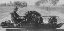
hinges in series. Draw the hinges as "cans" in series and do not be fussy about
the location of the cans which in principal are the same but in practice fan
out. First draw a hinge from the fixed space with the rotation axis along the
z-axis, second draw at the end of the first hinge a second hinge with the
rotation axis along the x-axis, and finally draw at the end of the second hinge
a third hinge with the rotation axis along the z-axis. The body fixed coordinate
system x'y'z' is located at the end of this third hinge. By considering the
intermediate coordinate systems between the three hinges you can derive the
rotation matrix R as a composition of three single rotation matrices about
principal axis as in x = R x', with R = R(phi) R(theta) R(psi). Note that these
Euler angles are no vectors since clearly the matrix multiplication is order
dependent, or in other words the individual Euler angles is non-commutative. By
the way, there are only 12 meaningfully ways of putting three orthogonal hinges
in series, so apart from the zxz Euler angles there are these 11 other ways to
parameterize R. Next I derived the expressions for the angular velocities omega in terms of
the Euler angles and the time derivatives of these angles by means of
differentiation of the identities R^T*R=I. I showed the formal way to derive
omega from Rdot*R^T but followed the intuitive way, by adding up the transformed
angular velocities of the hinges or "cans". This results in omega, w, in terms
of the Euler angles, e, and it's time derivatives edot as in w=A(e)*edot.
Next week continued.
Handed out homework Assignment 9 which
is due Thu 30 May 15:45 h.
Week 13
Thursday, 30 May 2013 15:45-17:30 u, room CT-CZ G.
-
Rotation Matrices, Euler Angles, and Euler Parameters.
We continued last
weeks subject on Euler Angles. We pick up were we left at the angular velocity
expressions. The rotational state of the system is defined by the Euler angles e
and the angular velocities w. The state equitation are the time derivatives of
these, so we need edot in terms of e and w. It turns out that the inverse of A is singular at the
Euler angle theta=0+k*pi. Which, looking at the cans in this configuration, is
obvious since the two rotation axis phi and psi are aligned! One way to
circumvent this problem is by redefining theta as theta=theta+pi/2, now the phi
and the psi axis are not anymore aligned. A major disadvantage of this method is
that the problem now is non-smooth in the state variables and we have to restart
our numerical integration procedure.
From Euler's theorem on Rotation,
"Any rotation in space can be represented as a rotation about a fixed axis at a
given angle", I derived the rotation matrix R in terms of the Euler parameters
lambda_0=cos(u/2) and lambda=sin(u/2)*h, where h is the axis of rotation with
unit length and u the angle of rotation. It turns out that R is bilinear in
lambda which is computational advantages. Think of the derivatives dR/dlambda=linear
in lambda and d2R/dlambda^2=constant! In the previous lectures we showed that R
can be represented by 3 independent parameters. Clearly the 4 Euler parameters
are dependent, namely the norm must be one: |lambda|=1. They live on this 4
dimensional unit sphere. In order to derive the expressions for the angular
velocities in terms of the Euler parameters and its time derivatives we start
again from Rdot*R^T=tilde(omega). After expansion we get the expressions 2*L*lamdadot=omega,
with matrix L linear in lambda. From this we like to solve lambdadot in terms of
lambda en omega. This can be done by adding the constraint on the lambdas in a
differentiated form, as in 2*lambdadot^T*lambda=0. The solution now becomes
lambdadot=1/2*L^T*[0; omega], note that this is without any singularities. This
is the main advantage of using Euler parameters. We also could have used
quaternion algebra to derive the various expressions. Euler parameters are unit
quaternions. In his pursued to multiply triplets Hamilton "invented" the
quaternion algebra. You can read all about this algebra in one of our recent
conference papers entitled "How to draw Euler angles and Utilize Euler
parameters", DETC2006Paper99307.pdf.
Handed out homework Assignment 10 which
is due Thu 6 June 15:45 h.
Bonus Question: Materialize the Euler angles by building "cans-in-series". Good for 1 Bonus point on HW10.
Thank you for the submissions to the last bonus question, which was: Materialize the Euler angles by building "cans-in-series". Below you find an impression of the submissions; Great Work! (one of you took the "cans-in-series" rather literally!)
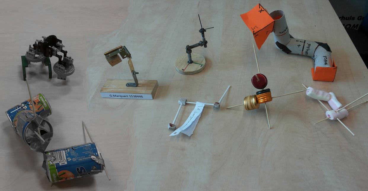
Materialization of Euler Angles, "Cans-In-Series" (click-on to enlarge).
Week 14
Thursday, 6 June 2013 15:45-17:30 u, room CT-CZ G.
-
Euler Parameters cont'd & Final Projects.
In the last lecture I presented two final projects:
- Final Project 1, Dynamic analysis of an Ejection Seat Reverse Bungee (average difficulty level).
- Final Project 2, Dynamic analysis of the motion of a bicycle, and notes on the bicycle project. (for die-hards!), this is an example of an uncontrolled stable bicycle, indeed very stable!.
You have to pick one final project. The final project is strictly individual. To get credit on the final project please do the following things:
-
On the top right corner neatly print the following, making appropriate substitutions as appropriate:
Sally Rogers, # 9123456
wb1443 Final Project
Due Mon Jan 24, 2005. - At the top clearly acknowledge all help you got from Faculty, students, or ANY other source (but for lecture and text). Examples could be "Mary Jones pointed out to me that I needed to draw the second FBD in problem 2." or "Nadia Chow showed me how to do problem 3 from start to finish." or "I basically copied this solution from the posted solutions." etc. If the TA thinks you are taking too much from other sources he/she will tell you. In the mean time don't violate academic integrity rules: be clear about which parts of your presentation you did not do on your own. More on academic integrity see: http://www.cuinfo.cornell.edu/Academic/AIC.html.
- All computer output should have your name clearly visible, as printed by the computer (e.g., title plots with your name, put your name in a comment in the first line of any .m files, etc.)
- Your work should be laid out neatly enough to read by someone who does not know how to do the problem. Part of your job as an engineer is not just to get the right answer, but convincingly so. That is your job on the final project as well.
Hand in your final project on paper in my paper mailbox. The due date is Monday 1 July 2013 17:00 h., which is three weeks from now. The graded work can be picked up at my office, again during office hours. There will be no oral exam. The final grade for the course will be 70% on the homework and 30% on the final project.
This was the last lecture.
You were a fine class, and it was a pleasure teaching this course this year!
Good Luck with the final project!
Did you enjoy Multibody Dynamics? Are
you intrigued by the dynamical behaviour of mechanical system? And you are
searching for a challenging and great MSc assignment?
Then please visit my
MSc project site; and
contact me if you
are interested in any of the projects or have an idea of a project of your own.
Week 15
Thursday, 13 June 2013 15:45-17:30 u, room CT-CZ G: NO LECTURE.